


One of the problems with predicting evolutionary outcomes is that the number of influencing factors is huge. Physics is a field of science where predictions can be very accurate - just think of sending rovers to Mars: the precision needed for that to succeed is daunting, and is a testament to the success of physics. However, this success stems from the simplicity of the physical systems that people have studied. Newton studied objects falling, which is a pretty simple thing with few factors influencing the outcome. The only relevant factor involved is gravitation, and it was fairly easy to achieve good predictability. The factors influencing the rover on its way to Mars are actually quite few as well. Biologists have a much harder time because the systems the first studied were so much more complex. Living things are just that much more complicated than a dead object falling (even if it is a living apple).
Evolution is driven by random changes to the genome and environmental factors. That's it. The problem is just that those are both highly unpredictable, whereas in physics things are easier. But here is the point I want to make: It's only easier in physics because physicists elect to study systems that are simple. There is a great joke where a physicist is able to predict the winner of any horse race to multiple decimal points - provided it was a perfectly elastic spherical horse moving through a vacuum (Wikipedia). Physicists don't contend with studying what is actually there in its messy reality, but instead reduce the problem to one that can be solved. Even though heating a pot of water involves many individual particles, boiling can be predicted with high accuracy, but only if it assumed that a meteor isn't going to crash the kitchen! Externalities are ignored and assumed not to happen. And that works well for physics, because that assumption is safe in many systems. But it is not safe at all in evolution.
The number of external effects that drive evolution is immense. But trying to predict evolution by starting with a model that includes everything is never going to work. First we must understand the simplest cases - in an approach identical to the one that has made physics so successful. We have to do this even if there is no system that actually evolves in this sort of vacuum in nature. Once we understand that system, we can build on it by adding more layers of complexity. Perhaps then one day mainstream biologists will be happy...
Population Size
The core entity of evolution is the population. It is the population that evolves, not the species or the individual. And the first thing to know about a population is its size, N. The size is the main determinant of what will happen to new mutations, such as the probability of fixation (i.e., the mutation existing in all individuals) and the strength of selection (governing whether a mutation will be under the influence of selection, or just genetic drift - note that there is always drift, which comes from the stochasticity (randomness) that is inherent in the evolutionary process, but sometimes it matters little compared to selection, which completely dominates in the case of an infinitely large population).
Mutation Rate
The second parameter to know is the rate at which new mutations appear, the mutation rate, µ. If there are no mutations (no more realistic in nature than an infinitely large population size), then evolution comes to a halt when genetic drift or natural selection has eliminated all variation. If µ is very large, the the population will experience a mutational meltdown and the loss fitness due to the accumulation of harmful mutations. The product of the population size and mutation rate is called the mutation-supply rate, µN. This quantity determines how many mutations occur: if it's low, then there are few mutations. In much of evolutionary theory it is assumed that the mutation-supply rate is so low that each mutation appears and goes to fixation (or most likely is lost) before the next mutation appears. This makes mathematics much easier, but it is not a realistic assumption. Rather, pretty much all natural populations have a mutation-supple rate large enough that there is always many different mutations present in the population. This is true for humans and for bacteria - and especially for viruses.
Lots of advances have been made in evolutionary theory (population genetics) given only these two parameters. But there is another that makes a huge difference, which describes what effect mutations have.
Fitness Landscape
The fitness landscape is a map where fitness is given as a function of the genotype or the phenotype. In other words, this function describes the expected reproductive success of every type of organisms in the population. If the fitness landscape is known, then the effect of every mutation is known, and it can be predicted statistically how the population will evolve. If the landscape is smooth (see Fig. 1) then there is only one outcome possible: the population will ascend the peak and then stay there. But if the landscape is rugged, then the population risks getting stuck on a local peak (at least for a very long time), or it may be fortuitous enough that it finds the global peak.

Figure 1. Smooth and rugged one-dimensional fitness landscapes. Both are simply fitness given as a function of either genotype or phenotype. Smooth landscapes have a single peak and the dynamics on it is very predictable: for non-zero mutations rates, the top of the peak will be located sooner or later. The only exception is if the mutation rate is very high, in which case all offspring have deleterious mutations that take them off the peak, aka as a mutational meltdown. The rugged landscape have multiple peaks separate by valleys of lower fitness. In the NK landscape rugged landscapes also have a greater range in fitness than smooth landscapes. This is an effect of pleiotropy, which in NK is coupled to the K-parameter, which determines the amount of genetic interaction. P.S. Not sure why I didn't indicate the axes here. Amateur! Again, it's fitness on the vertical axis, and genotype or phenotype on the horizontal axis. I could add, though, that a picture like this is more consistent with fitness as a function of a continuous phenotype (e.g., body size), while functions of genotype will most often be discrete. From Østman and Adami (2013).
Evolutionary dynamics in rugged landscapes are much harder to predict. That goes for the endpoint of evolution (the genotype or phenotype that the population ends at), which is easy to predict in smooth landscapes, and it is also true for the path that is taken. In one dimension the path is not hard to predict (if the population start to the left in the smooth landscape in Fig. 1, then it will move to the right until it hits the peak), but if there are many paths, then the situation is not so simple. If we look at the fitness landscape in Fig. 2A, which is reconstructed from Khan et al (2011), we see that there are many paths that can lead from genotype 00000 to 11111. Note that in this figure fitness is given for each of the 32 genotypes, but are plotted as a function of how many mutations away they are from the (arbitrarily chosen) 00000 genotype.
A population that starts at 00000 will end up on 11111, but it can take a number of routes there. Because the fitness gains are highest going through 00010 first, and then through 00110, 10110, 11110 to 11111, that route is most likely, but because evolution is a stochastic process (mutations are random and high fitness makes it more likely that you get to reproduce, but not certain), other routes are possible. In this example, Khan et al. actually found that the path taken was via 01000.

We can of course discuss the relevance of different paths. Does it really matter which path is taken? Where the population ends up seems more relevant, but suppose the population is a virus that we are fighting with anti-virals. In that case, we'd like to kill all the viruses, but if they evolve resistance, we could perhaps combat them with targeted drugs if we know which path they were going to take.
Figure 2B shows a rugged landscape with several peaks (at 11110, 11101, and 00000). If the population starts at 11111, it is most likely to go through 11110 and/or 11101. However, if the supply of mutations is low (WM, weak-mutaiton regime), the population risks getting permanently stuck there, and thus not able to locate the global optimum at 00000. By "permanently" I mean that the population will sit there for a very long time. Eventually it will move up, but it can take longer than other events that can change the landscape, and, if the fitness of those suboptimal genotypes are too low, the population can go extinct before they are able to escape to higher fitness. Fitness also affects population size, so that a population sitting on 11110 would in this case be about 10% lower than if it were sitting on 00000. In the simulation shown in Vid. 1 the population size is fixed at N=1,000, so this effect does therefore not occur. The mutation rate is very high, so the population is able to escape 11101 and 11110 by crossing the valley to reach 00000.
Video 1. Evolution in a rugged landscape. A population of 1,000 individuals evolving on a fitness graph all starting at genotype 11111. Mutation rate is 0.1 per generation (= chance to have one mutation; no double-mutations allowed here). The simulation is a Moran process (one individual is replaced by the offspring of another every update). The area of the circles are proportional to the number of individuals at that genotype.
One way to quantify how predictable evolution is is using information theory. The Shannon entropy was used by Szendro et al. (2013) to quantify how predictable evolution is in simulations of evolution in the Aspergillus niger fitness landscape (Fig. 3). One simply counts the frequency, pi, of each endpoint in a large number of replicate simulations (here, 100), and calculates the entropy as
 .
.
The lower the entropy S is, the higher predictability is. When all states are the same, pi=1, and S=0.
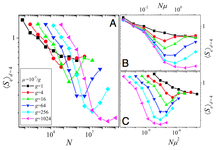
Evolution in smooth landscapes is very predictable (in terms of endpoints), while rugged landscapes can decrease predictability because the population can get stuck on different fitness peaks (which doesn't mean that a rugged landscape can cause speciation - for that, other factors are needed, like reproductive incompatibilities between different genotypes or negative frequency-dependent selection). Just as is seen in Fig. 3, increasing the mutation rate (up to a point) in rugged NK landscapes increases the chance that the population will find the global peak (Østman et al,, 2012).
Yes, we can predict evolution, but to achieve high predictability, certain conditions have to be met. A large mutation-supply rate helps, as does low ruggedness of the fitness landscape. So too does static landscapes; if the fitness landscape changes on time-scales comparable to the population dynamics, then predictability will suffer. There is very little research done on such dynamic fitness landscapes and how they affect evolutionary dynamics. One obvious question to tackle before answering this question is just how the landscape changes over time. Not much is known about this in natural populations, but it could be studied computational for different classes of changes, like peaks suddenly disappearing vs. more subtle changes in fitness values.
In summary, evolution is predictable if we know population size, mutation rate, and the fitness landscape.
References
Khan A, Dinh D, Schneider D, Lenski R, and Cooper T (2011). Negative Epistasis Between Beneficial Mutations in an Evolving Bacterial Population Science, 332 (6034), 1193-1196 DOI: 10.1126/science.1203801
Szendro IG, Franke J, de Visser JA, and Krug J (2013). Predictability of evolution depends nonmonotonically on population size. Proceedings of the National Academy of Sciences of the United States of America, 110 (2), 571-6 PMID: 23267075
Østman B and Adami C (2013). Predicting evolution and visualizing high-dimensional fitness landscapes in "Recent Advances in the Theory and Application of Fitness Landscapes" (A. Engelbrecht and H. Richter, eds.). Springer Series in Emergence, Complexity, and Computation (to appear). arXiv: 1302.2906v2